Article Text

Abstract
Family medicine has traditionally prioritised patient care over research. However, recent recommendations to strengthen family medicine include calls to focus more on research including improving research methods used in the field. Binary logistic regression is one method frequently used in family medicine research to classify, explain or predict the values of some characteristic, behaviour or outcome. The binary logistic regression model relies on assumptions including independent observations, no perfect multicollinearity and linearity. The model produces ORs, which suggest increased, decreased or no change in odds of being in one category of the outcome with an increase in the value of the predictor. Model significance quantifies whether the model is better than the baseline value (ie, the percentage of people with the outcome) at explaining or predicting whether the observed cases in the data set have the outcome. One model fit measure is the count-  , which is the percentage of observations where the model correctly predicted the outcome variable value. Related to the count-
  are model sensitivity—the percentage of those with the outcome who were correctly predicted to have the outcome—and specificity—the percentage of those without the outcome who were correctly predicted to not have the outcome. Complete model reporting for binary logistic regression includes descriptive statistics, a statement on whether assumptions were checked and met, ORs and CIs for each predictor, overall model significance and overall model fit.
- education
- epidemiology
- public health
Data availability statement
Data are available in a public, open access repository at https://github.com/jenineharris/logistic-regression-tutorial.
This is an open access article distributed in accordance with the Creative Commons Attribution Non Commercial (CC BY-NC 4.0) license, which permits others to distribute, remix, adapt, build upon this work non-commercially, and license their derivative works on different terms, provided the original work is properly cited, appropriate credit is given, any changes made indicated, and the use is non-commercial. See: http://creativecommons.org/licenses/by-nc/4.0/.
Statistics from Altmetric.com
Introduction
From its inception, the field of family medicine has prioritised patient care over research.1 However, research has an important place in family medicine to improve quality, responsiveness and innovation in patient care.2 As a result, there have been numerous calls in recent years3 for family and community medicine practitioners around the world4 5 to become more involved in research.6 Among the recommendations for improving family medicine research is strengthening the use of appropriate research methods.6
Binary logistic regression is one method that is particularly appropriate for analysing survey data in the widely used cross-sectional and case–control research designs.7–9 In the Family Medicine and Community Health (FMCH) journal, 35 out of the 142 (24.6%) peer-reviewed published original research papers between 2013 and 2020 reported using binary logistic regression as one of the analytical methods. Given the high percentage of FMCH publications that include binary logistic regression, understanding this method is important for FMCH authors and reviewers.
The binary logistic regression model is part of a family of statistical models called generalised linear models. The main characteristic that differentiates binary logistic regression from other generalised linear models is the type of dependent (or outcome) variable.10 A dependent variable in a binary logistic regression has two levels. For example, a variable that records whether or not someone has ever been diagnosed with a health condition like lung cancer could be measured in two categories, yes and no. Likewise, someone might have coronary heart disease or not, be physically active or not, be a current smoker or not, or have any one of thousands of diagnoses or personal behaviours and characteristics that are of interest in family medicine.
In addition to a binary dependent variable, a binary logistic regression has at least one independent variable that is used to explain or predict values of the dependent variable. For the example of lung cancer diagnosis, some logical independent variables could be age or smoking status. People who are smokers have higher odds of lung cancer, as do people who are older. Unlike the dependent variable, independent variables are not limited to be binary and can have two or more categories or be continuous.
There are many ways to identify and select variables that are important to include in a logistic regression model and researchers should carefully consider which variables to include. Some suggested strategies for variable identification and selection in logistic regression are included in a 2019 paper by Shipe et al11 and other strategies for selecting variables are included in a 2018 paper by Heinze et al.12 For those researchers new to logistic regression, collaboration with experienced researchers or methodologists is recommended.6
The following sections are a step-by-step demonstration of how to conduct and interpret a binary logistic regression model. The analyses in this paper were conducted in R V.4.1.113 using the following packages: tidyverse,14 odds.n.ends,15 car,16 finalfit,17 knitr18 and table 1.19 The statistical code for reproducing the results or for adapting the code to use to conduct analysis on other data is available at this URL: https://github.com/jenineharris/logistic-regression-tutorial
Step 1: exploratory data analysis
Before a binary logistic regression model is estimated, it is important to conduct exploratory data analysis (EDA). EDA can include descriptive statistics and/or graphs. EDA serves multiple purposes, including: confirmation that the data were measured and labelled correctly, identification of potential problems with data distributions (eg, no cases in an important category), a preview of what model results might show, and information that can be used in reproducing statistical results.20
As an example, consider a small data set with the survey responses of 32 long-term smokers. The data set includes three variables: lungCancer, yearsSmoke and bmi. The lungCancer variable is an indicator of whether the survey participant has ever been diagnosed with lung cancer; it has a value of 1 for yes and 0 for no. The years smoke variable is the number of years the survey participant has been a smoker, and the bmi variable is the category of body mass index (BMI) that the participant is in, which includes two categories: underweight or normal BMI and overweight or obese BMI. If the goal is to build a logistic regression model from these data where lung cancer diagnosis is the outcome variable and is predicted by years of smoking and BMI category, the first step would be to conduct EDA that first explores each variable and then explores the intersection of each predictor with the lung cancer outcome variable.
One way to explore each variable separately before modelling is to produce a table of descriptive statistics, choosing the most appropriate statistics for each variable type. Since years of smoking is closer to being continuous variable (rather than categorical), the best descriptive statistics would be either mean and SD or median and IQR. The way to choose between these two options is to determine whether the years of smoking data are normally distributed or not. Continuous variables that are relatively normally distributed are best described by mean and SD while those that are not normally distributed are more appropriately described by median and IQR.
The histogram (figure 1) suggests that the variable is right skewed rather than normal, so median and IQR would be a more appropriate choice for descriptive stats for the years smoke variable. The other two variables, bmi and lungCancer are both categorical, so the most appropriate descriptive statistics are percentages and frequencies. Table 1 shows an example of a useful data exploration prior to binary logistic regression modelling.
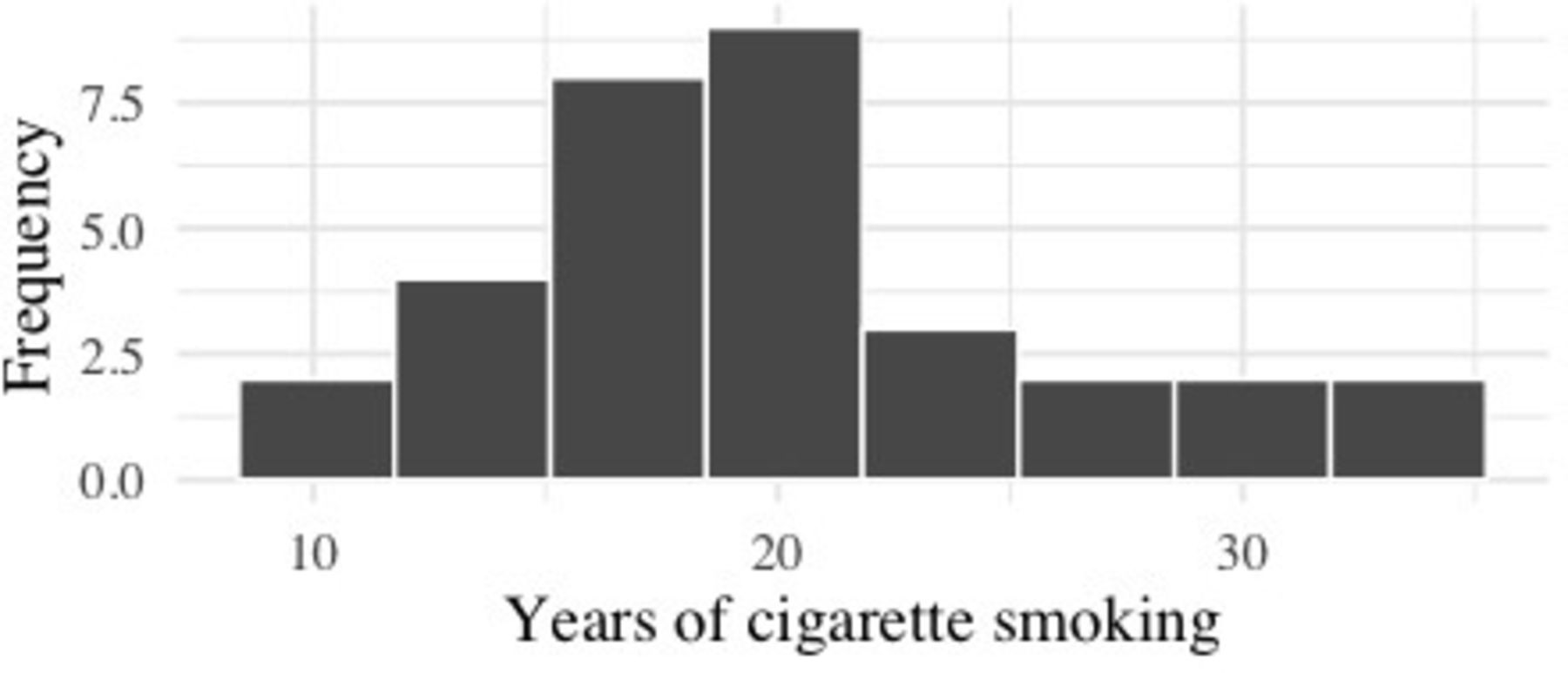
Histogram showing distribution of years smoking for a sample of 32 smokers.
Example table showing characteristics of people in a small data set (n=32)
Table 1 shows that fewer than half of participants had ever been diagnosed with lung cancer, about 40% are overweight, and the median number of years smoking is just over 19. At this point, if something in the descriptive statistics seemed inconsistent with what you know about the sampling or the measurement, you could review the data and any data management steps to ensure everything was correctly recorded and labelled. Once satisfied with the univariate descriptive statistics, the next step might be computing descriptive statistics by outcome group. This step provides some insight into what the statistical modelling might find.
It is clear from table 2 that the people in the data who were diagnosed with lung cancer were smokers for a higher median number of years. It also appears that the distribution of people across BMI groups is different for the lung cancer and no lung cancer groups. For those without lung cancer, a higher percentage were in the underweight or normal BMI group and fewer in the overweight or obese BMI group compared with people being evenly split into these two BMI groups for those participants with lung cancer.
Example of a stratified table showing characteristics of people by lung cancer status in a small data set (n=32)
Tables 1 and 2 provide a few pieces of information useful for the regression modelling. First, the data seem to be cleaned and appropriately labelled. Second, the data suggest that model could show that the odds of lung cancer is higher with more years of smoking. The model might also find higher odds of lung cancer in those who are overweight or obese compared with underweight or normal BMI, but this is less clear from the descriptive analyses. If the model results are very different from what the descriptive statistics suggest will happen, it is worth taking the time for further exploration of the data to ensure there are no mistakes in recording and managing it correctly and the model settings are as expected.
Step 2: check binary logistic regression assumptions
Statistical models like binary logistic regression are developed with certain underlying assumptions about the data. Assumptions are features of the data that are required for the model to work as expected and, when one or more assumptions are not met, the model may produce misleading results. For example, consider the mean as a basic statistical model. The mean is one way to explain where the middle is in a set of continuous numbers. For the mean to work as intended and produce a value that is in the middle, the numbers are assumed to follow a normal distribution. If the numbers are skewed to the right, like the years of smoking variable in figure 1, the calculated mean will be higher than the centre of the data. If the numbers are skewed to the left, the calculated mean will be lower than the centre of the data. With non-normal data, a different model, like the median, is likely to be a more accurate measure of central tendency.
Binary logistic regression relies on three underlying assumptions to be true:
The observations must be independent.
There must be no perfect multicollinearity among independent variables.
Continuous predictors are linearly related to a transformed version of the outcome (linearity).
Before conducting a logistic regression analysis, check these three assumptions. The model must meet all assumptions to be reported as unbiased and generalisable outside the sample.
Checking the assumptions
The independence of observations assumption requires that each of the observations in a data set is unrelated to the other observations in the data set. There are at least two different ways that data commonly fail this assumption. The first way is that a data set includes multiple observations from the same person (or mouse, or organisation, or whatever the type of observation is). The second way is where data include some sort of grouping like multiple family members who live in the same residence, multiple people from the same class in a school, or several people who live close together in the same neighbourhood. When people are in the same family, class or neighbourhood, they are more likely to share characteristics, which can limit the amount of variability in the data and introduce bias into the results. Checking this assumption requires knowing how the data were collected to ensure that the observations are unrelated.
The no perfect multicollinearity assumption requires that the independent variables are not perfectly correlated with each other. Variables that are highly, or perfectly, correlated with each other are statistically measuring the same thing (or similar things) and so are essentially redundant. Including variables in a model that are redundant can result in unstable model results. Correlation coefficients are often used to check for correlation among independent variables; two variables that are correlated at r=0.7 or higher share 49% or more variance and are considered somewhat redundant and problematic to include together in a single model as separate independent predictors.
There are several ways of checking the no perfect multicollinearity assumption. One that is commonly used is the Variance Inflation Factor or VIF. The VIF score for a variable quantifies how well that variable is explained by the other variables in the model. For binary logistic regression, the VIF score is generalised (GVIF) and takes on larger values.21 To use the GVIF in a similar way as the VIF, a new value is often computed:  . Although there does not seem to be consensus on a cut-off value for the
  , one commonly used cut-off for the
  is two. If this is used, variables with a
  value of two or higher might be considered problematic while those with
  less than two do not have any multicollinearity problems. In R, the vif() function in the car package prints the
  for logistic regression models. The output gives the value for each variable, like this:
## yearsSmoke bmi
## 1.783835 1.783835
The two  values are below two and so are not problematic. For this model, the no perfect multicollinearity assumption is met.
The linearity assumption requires that continuous independent variables, or predictors, have a linear relationship with the log-odds of the predicted probabilities for the outcome. Linear relationships are relationships that seem to follow a relatively straight line. One way to check this relationship is to create a scatterplot with the continuous predictor on the x-axis and the log-odds of the predicted probabilities on the y-axis. Add a loess curve and a line representing a linear relationship between the two variables to the scatterplot. The loess curve shows the relationship between the predictor and the transformed outcome in a more nuanced way, while the fitted line shows what the relationship between the two would be if it were linear. If the loess curve and the fitted line are approximately the same, the linearity assumption is met. If the loess curve deviates from the line, the linearity assumption fails.
The loess curve is very close to the linear relationship so the linearity assumption appears to be met (figure 2). Assuming that these data were collected using an acceptable sampling frame without related observations (independence of observations assumption), the data meet the assumptions to report the model as unbiased.

Checking the linearity assumption graphically.
Step 3: estimate the binary logistic regression model
The dependent variable for binary logistic regression is a categorical variable with two categories (denoted as y in equation 1). In the statistical model it is transformed using the logit transformation into a probability ranging from 0 to 1 (equation 1).
Equation 1. A statistical form of the binary logistic regression model.

In equation 1, the p(y) stands for the probability of one category (often the presence of a behaviour or condition) of the dependent variable y, the b are coefficients of the independent variables or predictors, and the x are the independent variables. Those who are familiar with linear regression might notice that the statistical form of the linear regression model is inside the parentheses of the exponent of e in the denominator of the right-hand side of the equation.
Visualising the logistic function can help to clarify why this statistical form is useful for examining a binary outcome. Figure 3 shows the logistic function as the curve connecting the data points. Each data point is plotted with a value of the outcome along the y-axis. Because the outcome is binary with the two values of 0 and 1, the points are plotted at y=0 and y=1. The predictor variable is shown along the x-axis and appears to be continuous. Each data point takes a value of x which seems to range from about 10 to about 35. It is clear that the data points in the y=0 category of the outcome generally have lower values of x than the data points in the y=1 category. This pattern suggests that, as x increases, the probability of a person having the outcome value of y=1 also increases.
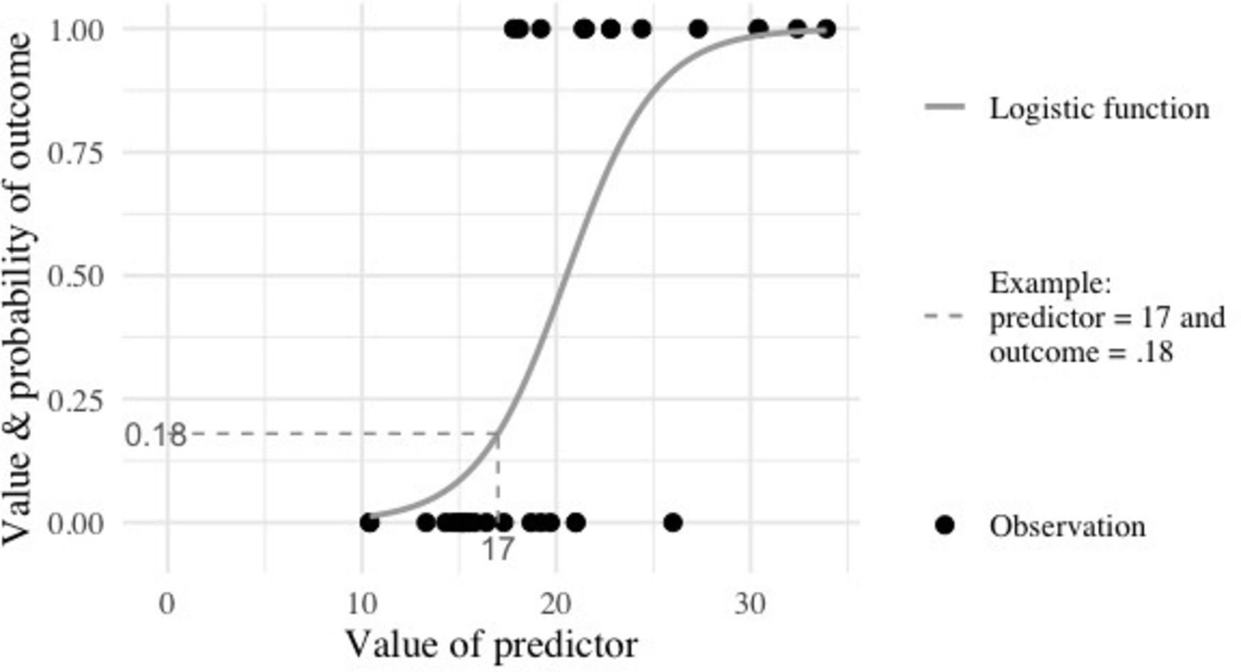
The logistic function with example data.
The grey logistic function line is the logistic regression model for these data. The line identifies the predicted probability of y=1 for each value of x. For example, if x=17, the predicted probability of y would be .18. This might be translated into into a percentage with a statement like, there is an 18% probability that someone with an x value of 17 would have a y value of 1. A more concrete example might be to think of the x value as years a person has smoked cigarettes daily and y as their probability for being diagnosed with lung cancer. So, a person who has smoked daily for 17 years has an 18% probability of being diagnosed with lung cancer. Please note that these data are not actual lung cancer data; this is just an example to assist in developing intuition around the logistic function meaning. If these data were years of smoking predicting lung cancer diagnosis, equation 1 might be rewritten as equation 2:
Equation 2. Applying the statistical form of the binary logistic regression model.

Step 4: compute ORs and report the results
While the predicted probabilities from the logistic function can be useful in measuring how well the model is predicting or explaining the outcome, the results of logistic regression are usually reported with ORs and CIs. Similar to the interpretation of a coefficient in linear regression, ORs quantify the change in the odds of having the outcome (ie, the odds that an observation has the value of 1 for the outcome variable) with a one-unit change in the predictor. Odds are computed using probabilities (equation 3).
Equation 3. Computing odds from probabilities.

Because the logistic function is used to compute probabilities (see figure 1), add the logistic model from equation 1 into equation 3 to get equation 4 showing how odds are computed for a logistic regression model.
Equation 4. Computing odds from a logistic regression model.

Once the  and
and  are estimated using a statistical software package like SAS, R or SPSS, these values can be substituted into the simplified version of equation 4 to compute odds. This is not the final step, however, since odds and ORs are different. An OR is a ratio of two odds and is computed by dividing the odds of the outcome at one value of a predictor by the odds of the outcome at the previous value. So, for example, to compute the OR for lung cancer in our previous example, divide the odds of someone who has smoked for 15 years by the odds for someone who has smoked for 14 years. The result will be the increased or decreased odds of lung cancer with every 1 year increase in age. Equation 5 shows the statistical form of this computation.
Equation 5. Using odds to compute ORs from a logistic regression model.

As an example, consider the output from R showing the estimates for the regression model used in figure 2.
##
## Call:
## glm(formula=lungCancer ~ (yearsSmoke), family=binomial(“logit”),
## data=lungCancerData)
##
## Deviance Residuals:
## Min 1Q Median 3Q Max
## −2.2127–0.5121 −0.2276 0.6402 1.6980
##
## Coefficients:
## Estimate SE z value Pr(>|z|)
## (Intercept) −8.8331 3.1623 –2.793 0.00522 **
## yearsSmoke 0.4304 0.1584 2.717 0.00659 **
## ---
## Signif. codes: 0 '***' 0.001 '**' 0.01 '*' 0.05 '.' 0.1 ' ' 1
##
## (Dispersion parameter for binomial family taken to be 1)
##
## Null deviance: 43.860 on 31 degrees of freedom
## Residual deviance: 25.533 on 30 degrees of freedom
## AIC: 29.533
##
## Number of Fisher Scoring iterations: 6
The coefficient for years smoking is 0.4304. Substitute this value into equation 5,  , to get an OR of 1.54. So, for every 1 year increase in time spent as a smoker, the odds of lung cancer for a participant in our sample are approximately 1.54 times higher. While the OR is useful to understand the direction and magnitude of the relationship between a predictor and the outcome, more information is needed to understand whether the OR for the sample suggests a relationship in the population that the sample came from. To understand this, a 95% CI is typically computed and reported with each OR.
A 95% CI for an OR shows the range of values where the true population value of the OR likely lies. That is, if 100 samples were selected from the population and a 95% CI were computed using the data from each sample, 95 of those CIs would contain the true value of the OR (given appropriate research practices). Most statistical software packages compute 95% CIs with ORs as part of the logistic regression output. For example, the lung cancer model output might look like this:
## (Intercept) 0.0001458295 0.00000005391304 0.02024744
## yearsSmoke 1.5378933421 1.20314425841351 2.28063266
This output includes the 1.54 OR for years of smoking along with the 95% CI 1.2 to 2.28. So, the odds of lung cancer increase by approximately 1.54 times for every year longer a participants smokes and, in the population that this sample came from, the true OR likely lies between 1.20 and 2.28. Because the range of the 95% CI does not include 1, this indicates that the OR is statistically significantly different from 1. If the CI had included 1, the OR would not be statistically significantly different from 1. An OR of 1 indicates that there is no difference in odds. So, for example, someone with 14 years of smoking would have no higher nor lower odds of lung cancer than someone with 15 years of smoking if the 95% CI for the OR included 1.
A logistic regression model with a single predictor in it produces unadjusted ORs demonstrating the relationship between the predictor and the outcome without taking into account other independent predictors or confounding variables. Reporting the unadjusted ORs for the main predictor or predictors of interest may contribute to understanding how covariates influence the relationship between the predictor and outcome.22 23
Logistic regression models can also include categorical predictors. For example, adding a BMI variable with two categories, underweight or normal BMI and overweight or obese BMI, to the lung cancer model results in the following output:
## (Intercept) 0.000003035556 0.00000000001397127 0.003054554
## yearsSmoke 1.975695580376 1.35547578843285321 3.860461189
## bmiOverwei 0.049426238402 0.00109959322745114 0.739726723
Both of the CIs indicate that the association between the predictor and lung cancer is statistically significant. For every additional year of smoking, the odds of lung cancer are approximately 1.98 times higher (95% CI 1.36 to 3.86). Compared with people in the under or normal weight BMI group, those who are classified as having an overweight or obese BMI have approximately 0.05 times the odds of having lung cancer (95% CI 0.001 to 0.74). When an OR is less than one, another way to report the OR is to subtract the value from one and report the result as a percent decrease in odds, like this: Compared with people in the under or normal weight BMI group, those who are classified as having an overweight or obese BMI have approximately 95.06% lower odds of having lung cancer (95% CI 0.001 to 0.74). Remember that the data shown here are for demonstration purposes only and these model results should not be taken as true relationships between the predictors and lung cancer.
Model significance and model fit
In addition to reporting the results of assumption checking and the ORs and CIs, the model significance and model fit are useful tools to understand how well your model is reflecting what was observed in the data. First, model significance determines if your model explains the data better than the baseline percentage of people with the outcome would explain the data. Model significance is determined by a χ2 statistic that is computed by comparing a null model that has no predictors in it (and thus is the percentage of people with the outcome of interest) to the model with predictors in it. The χ2 statistic is computed by taking the probability of the outcome and subtracting the value of the outcome for each participant. So, with the lung cancer data, the percentage of people who have lung cancer is 43.75%, so the predicted probability for each person in the data set to have lung cancer would be 0.4375. This value is subtracted from each person’s actual value for the outcome (0 or 1) and the result is squared. All of these squared values are then added up into a value called Null Deviance. The Null Deviance quantifies how far the predicted probabilities from a model with no predictors (null model) were from the true values of the outcome. The same process is then repeated for the predicted probabilities from the model with predictors. This is the model deviance.
The difference between the null deviance and the model deviance follows a χ2 distribution with the number of df being the number of coefficients in the model. If the χ2 is statistically significant, this indicates that the model is doing a significantly better job at predicting the probability that someone has the outcome compared with just using the percentage of people with the outcome as a model. Most statistical software will provide the model χ2 and its significance. For example, the R package odds.n.ends gives model significance like this:
## 23.214 2 <0.001
The model using BMI category and years of smoking to explain lung cancer status is statistically significantly better than the baseline at predicting lung cancer status [  (2)=23.214; p<0.001].
While model significance suggests whether a model is better than the baseline percentage of people with the outcome, model fit metrics are useful for knowing how much better than the baseline a model is at predicting the values of the outcome. One way to understand model fit for binary logistic regression is to compute the percentage of observed values of the outcome that your model correctly predicted. The contingency table used here computes predicted probabilities based on the model and then classifies the probabilities using a cut-off of 0.5. So, any predicted probability of 0.5 or greater is classified as having the outcome and any predicted probability below 0.5 is classified as not having the outcome. With the lung cancer example, what percentage of people who had lung cancer were predicted to have lung cancer and what percentage of people without were predicted to be without. An examination of the contingency table, or the table showing observed and predicted values, can help understand how well the model did in explaining the observed data (table 3).
Contingency table showing observed and predicted values of the outcome for the lung cancer model
The contingency table shows 15 people who did not have the outcome (observed=0) were correctly predicted to not have the outcome (predicted=0). Three people who did not have the outcome (observed=0) were incorrectly predicted to have the outcome (predicted=1). Ten people who had the outcome were correctly predicted, while four people who had the outcome were incorrectly predict. Altogether, 15+10 or 25 of the 32 observations had the outcome correctly predicted by the model for a per cent correctly predicted of 78.12%. So, for 78.12% of the people in the data set used to estimate the lung cancer model, the model then correctly predicted whether or not the participants had lung cancer.
The overall per cent correctly predicted gives a sense of how well the model did explaining or predicting the value of the outcome for all the participants. Sometimes it might be valuable to know how well the model did for those with the outcome or how well it did for those without the outcome. The term for how well a model predicts those with the outcome is sensitivity while specificity is how well the model predicts those without the outcome. In this case, 10 out of 14 of the people with lung cancer were correctly identified by the model for a sensitivity of 0.714 or 71.4%. The specificity of the model was higher, with 15 out of 18 (83.3%) of people without the outcome correctly predicted by the model.
Summary
The final model report should include:
Descriptive statistics on the outcome variable and each of the predictors.
Information on which assumptions were checked and whether they were met.
A statement about model significance.
A statement about model fit.
The model estimates including ORs and their 95% CIs.
An interpretation of the findings.
As an example, the lung cancer model shown here might be reported as follows:
We used binary logistic regression to examine whether years of smoking and BMI helped to explain lung cancer diagnosis in a sample of 32 people. The sample include 14 people with lung cancer and 18 without. The data met the binary logistic regression assumptions of independent observations, no perfect multicollinearity, and a linear relationship between the continuous predictor (years smoking) and the logit of the outcome. The model was statistically significantly better than the baseline at explaining lung cancer status [
(2)=23.214; p<0.001] and correctly predicted the lung cancer status of 78.1% of participants include 71.4% of those with lung cancer and 83.3% of those without. Model estimates suggested that, for every additional year of smoking, the odds of lung cancer are approximately 1.98 times higher (95% CI 1.36 to 3.86). In addition, compared with people in the under or normal weight BMI group, those who are classified as having an overweight or obese BMI have approximately 0.05 times the odds of having lung cancer (95% CI 0.001 to 0.74).

ORs and CIs are often reported in tables for larger models, but for a model with just a few predictors, including the ORs and CIs in the text provides the same information and uses less space.
Researchers using logistic regression should note that logistic regression results, regardless of the size, direction or significance of the ORs, do not imply a causal relationship between the predictors and the outcome.24 Also, while this tutorial describes the basics of conducting and reporting a logistic regression analysis, there are many more details to know about these models and their appropriate uses.7–9 25–27
Data availability statement
Data are available in a public, open access repository at https://github.com/jenineharris/logistic-regression-tutorial.
Ethics statements
Patient consent for publication
Ethics approval
This study does not involve human participants.
References
Footnotes
Twitter @jenineharris
Contributors JKH is the guarantor of this work and conceptualised and developed all aspects of this paper.
Funding The authors have not declared a specific grant for this research from any funding agency in the public, commercial or not-for-profit sectors.
Competing interests None declared.
Provenance and peer review Not commissioned; externally peer reviewed.